
Dates and times
Last updated on 2026-04-28 | Edit this page
Estimated time: 0 minutes
Overview
Questions
What is the duration of an event?
How can I view trends in measurements?:
Objectives
Know that dates and times are used in most tables in the OMOP CDM to record when events happened.
Understand that dates and times are often used in pairs to record the start and end of an event, which allows us to calculate the duration of that event.
Know how to convert a date or datetime string to a date or datetime object in R.
Introduction
This episode considers dates and times in the OMOP Common Data Model (CDM).
For this episode we will be using a sample OMOP CDM database that is pre-loaded with data. This database is a simplified version of a real-world OMOP CDM database and is intended for educational purposes only.
(UCLH only) This will come in a similar form as you would get data if you asked for a data extract via the SAFEHR platform (i.e. a set of parquet files).
As part of the setup prior to this course you were asked to download
and install the sample dataset. If you have not done this yet, please
refer to the setup instructions. For now, we
will assume that you have the sample OMOP CDM dataset available on your
local machine at the following path: ./data/omop/ and the
functions in a folder ./code/parquet_dataset.
You will then need to load the database as shown in the previous episode.
R
library(dplyr)

open_omop_dataset <- function(path) {
    # iterate over table level directories
    list.dirs(path, recursive = FALSE) |>
      # exclude folder name from path and use it as index for named list
      purrr::set_names(~ basename(.)) |>
      # "lazy-load" list of parquet files from specified folder
      purrr::map(arrow::open_dataset)
}
R
omop <- open_omop_dataset("./data/omop")
and the useful functions we created in the previous episode to look up concept names and ids.
R
get_concept_name <- function(omop_obj, id) {
  omop_obj$concept |>
    filter(concept_id == id) |>
    select(concept_name) |>
    collect()
}
R
get_concept_id <- function(omop_obj, name) {
  omop_obj$concept |>
    filter(concept_name == name) |>
    select(concept_id) |>
    collect()
}
Dates and times in OMOP
Dates and times are used in most tables to record when events
happened, usually with the start and end date recorded. In many places
there is also a time component, for example to record the time of day
when a measurement was taken. Column names are frequently either
suffixed with _date or _datetime to indicate
whether they contain just a date or both date and time information.
Parquet has data types for dates and date-times, but if the data was
written to CSV or as a string then we can convert these strings to date
or datetime objects using the as.Date() or
as.POSIXct() functions, respectively. This will allow us to
perform date and time calculations and visualizations more easily.
Usually the dates come in pairs, for example
condition_start_date and condition_end_date in
the condition_occurrence table. This allows us to determine
the duration of a condition, for example, by calculating the difference
between the start and end dates.
Challenge
Using the condition_occurrence table, display the
duration in days for each condition and find the average duration of
conditions in this dataset.
R
# First we need to read in the condition_occurrence table with only the columns we need to worry about and collect the data into memory
condition_occurrence <- omop$condition_occurrence |>
  select(condition_occurrence_id, condition_start_date, condition_end_date) |>
    collect()

# Exclude any rows where the end date is missing, as we can't calculate the duration for these
condition_occurrence <- condition_occurrence |>
    filter(!is.na(condition_end_date))

# We can calculate the length of each condition in days by taking the difference between the end date and the start date. We add 1 to include both the start and end date in the duration calculation.
condition_occurrence <- condition_occurrence |>
  mutate(
    length_days_inclusive = as.integer(condition_end_date - condition_start_date) + 1L
  )

# Finally we can calculate the average duration of conditions in this dataset, excluding any missing values
average_duration <- mean(condition_occurrence$length_days_inclusive, na.rm = TRUE)

average_duration
OUTPUT
[1] 3.178571Answer: The average duration of conditions in this dataset is approximately 3.2 days.
CODING NOTE: In the code above, we first read in the
condition_occurrence table and selected only the relevant
columns. We then filtered out any rows where the
condition_end_date was missing, as we cannot calculate the
duration for these conditions. Next, we calculated the length of each
condition in days by taking the difference between the end date and the
start date and adding 1 to include both the start and end date in the
duration calculation. Finally, we calculated the average duration of
conditions in this dataset by taking the mean of the
length_days_inclusive column, excluding any missing
values.
It is not uncommon for the end date to be missing in the data, for example if a condition is ongoing at the time of data extraction. In this case, we can only calculate the duration for conditions that have an end date recorded.
Also consider the measurement table where we have both a
measurement_date and a measurement_datetime
column. The measurement_date column contains just the date
of the measurement, while the measurement_datetime column
contains both the date and time of the measurement. Depending on the
analysis we want to do, we may choose to use one or the other of these
columns. Note generally a measurement doesn’t have a start and end date,
but just a single date or datetime when the measurement was taken.
Challenge
Using the measurement table, graph the
Body temperature of patient 113 over time. You
can use either the measurement_date or
measurement_datetime column for the x-axis.
R
library(ggplot2)
# First we need to know the concept id for body temperature
get_concept_id(omop, "Body temperature")
OUTPUT
# A tibble: 1 × 1
  concept_id
       <int>
1    3020891
R
# Then we need to read in the measurement table, filter for the measurements of interest and collect the data into memory
measurement <- omop$measurement |>
    filter(person_id == 1113 & measurement_concept_id == 3020891) |>
    collect()

ggplot(measurement, aes(x = measurement_datetime, y = value_as_number)) +
  geom_point() +
  geom_line() +
  labs(
    title = "Body temperature of patient 113 over time",
    x = "Date and time of measurement",
    y = "Body temperature (°C)"
  )
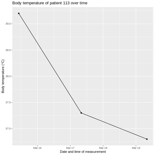
CODING NOTE: In the code above, we first used the
get_concept_id() function to find the concept ID for “Body
temperature”. We then read in the measurement table and
filtered for measurements of patient 113 with the relevant
concept ID. We collected this data into memory. Finally, we created a
line plot of body temperature over time using ggplot2, we
did not need to order the data by datetime as ggplot does this for us
when we set the datetime column as the value for the x-axis.
Converting data types
We are working with a dataset from parquet files which contains information about the data type of each column. If you are working with a csv file as an input, then there are no guarantees that a dataset will have the expected data types. We can simulate what this may look like by creating a new measurement table that has string types instead of the expected types.
R
measurement_to_fix <- omop$measurement |>
  mutate(
    across(c(measurement_datetime, measurement_date, value_as_number), ~ as.character((.x)))
    ) |>
  collect()

measurement_to_fix
OUTPUT
# A tibble: 353 × 12
   measurement_id person_id measurement_concept_id measurement_date
            <int>     <int>                  <int> <chr>
 1           8001      1111                3020891 2025-07-22
 2           8002      1111                3004249 2025-07-22
 3           8003      1111                3012888 2025-07-22
 4           8004      1111                3027018 2025-07-22
 5           8005      1112                3013502 2024-01-15
 6           8006      1112                3027018 2024-01-15
 7           8007      1112                3020891 2024-01-15
 8           8009      1112                3027315 2024-01-16
 9           8010      1112                3013502 2024-01-18
10           8011      1112                3013502 2025-12-24
# ℹ 343 more rows
# ℹ 8 more variables: measurement_datetime <chr>, operator_concept_id <int>,
#   value_as_number <chr>, value_as_concept_id <int>, unit_concept_id <int>,
#   range_low <dbl>, range_high <dbl>, visit_occurrence_id <int>
We’ve used the across() function from the
dplyr package to apply the as.character()
function to three columns.
Challenge
Using the measurement_to_fix table.
- Calculate the number of days between the first and last
Body temperaturemeasurement for each patient, sorting the final output bypatient_id. Which patient hasBody temperaturemeasurements spanning mulitple days? - Create a scatter plot of all
Systolic blood pressureandDiastolic blood pressuremeasurement values that were taken between the 1st of January 2025 and 1st of October 2025, usingmeasurement_datetimefor the x-axis. Colour the points by thepatient_id.
- Calculate the number of days between the first and last
Body temperaturemeasurement for each patient, sorting the final output bypatient_id. Which patient hasBody temperaturemeasurements spanning mulitple days?
R
# Convert the date column to a date
measurement_with_date <- measurement_to_fix |>
    mutate(measurement_date = as.Date(measurement_date, format = "%Y-%m-%d"))

# Calculate the number of days between first and last body temperature measurement
measurement_with_date |>
  filter(measurement_concept_id == 3020891) |>
  summarise(
    first_measurement_date = min(measurement_date),
    last_measurement_date = max(measurement_date),
    days_between = as.integer(last_measurement_date - first_measurement_date),
    .by = person_id
    ) |>
  arrange(person_id)
OUTPUT
# A tibble: 5 × 4
  person_id first_measurement_date last_measurement_date days_between
      <int> <date>                 <date>                       <int>
1      1111 2025-07-22             2025-07-22                       0
2      1112 2024-01-15             2024-01-15                       0
3      1113 2025-03-15             2025-03-19                       4
4     34567 2025-12-28             2025-12-28                       0
5     78901 2004-09-15             2004-09-15                       0
Answer: Only patient 113 has
Body Temperature measurements over multiple days.
CODING NOTE: In the code above, we converted the
measurement_date from character to date instances using the
as.Date() function. We then filtered the data to the
concept for Body Temperature, and used summarise() grouped
by person_id to calculate the first and last measurement
date, and their difference in numbers of days.
- Create a scatter plot of all
Systolic blood pressureandDiastolic blood pressuremeasurement values that were taken between the 1st of January 2025 and 1st of October 2025, usingmeasurement_datetimefor the x-axis. Colour the plot by thepatient_id.
R
# Correct the data types of remaining columns
measurement_fixed <- measurement_with_date |>
  mutate(
    measurement_datetime = as.POSIXct(measurement_datetime, tz = "UTC"),
    value_as_number = as.double(value_as_number)
  )

# Get concepts for blood pressure
systolic_concept <- get_concept_id(omop, "Systolic blood pressure") |>
  pull()

diastolic_concept <- get_concept_id(omop, "Diastolic blood pressure") |>
  pull()

# Filter measurements by concepts and time range
measurement_fixed |>
  filter(
    measurement_concept_id %in% c(systolic_concept, diastolic_concept),
    measurement_datetime >= "2025-01-01",
    measurement_datetime < "2025-10-01",
  ) |>
  ggplot(aes(x = measurement_datetime, y = value_as_number, colour = as.factor(person_id))) +
  geom_point() +
  labs(
    title = "Blood pressure measurements over time",
    x = "Measurement taken (datetime)",
    y = "Blood pressure",
    colour = "person_id"
  )
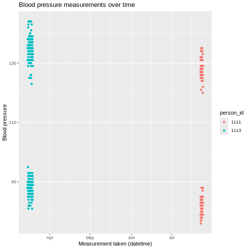
CODING NOTE: In the code above, we converted the
measurement_datetime from character to datetime instances
using the as.POSIXct() function, we would need to confirm
which timezone the data is in if we haven’t already been told. We also
converted the value_as_number column to a double (numeric
allowing for decimal places) data type using as.double().
We then found the concepts required, filtered to these and the date
range and used these to plot the data using ggplot(). We
used the colour option in aes() to define that
the colour of the points should be, converting it to a factor using
as.factor() so that the continuous variable is diplayed as
categories.
Dates and times are used in most tables in the OMOP CDM to record when events happened.
They are often used in pairs to record the start and end of an event, which allows us to calculate the duration of that event.